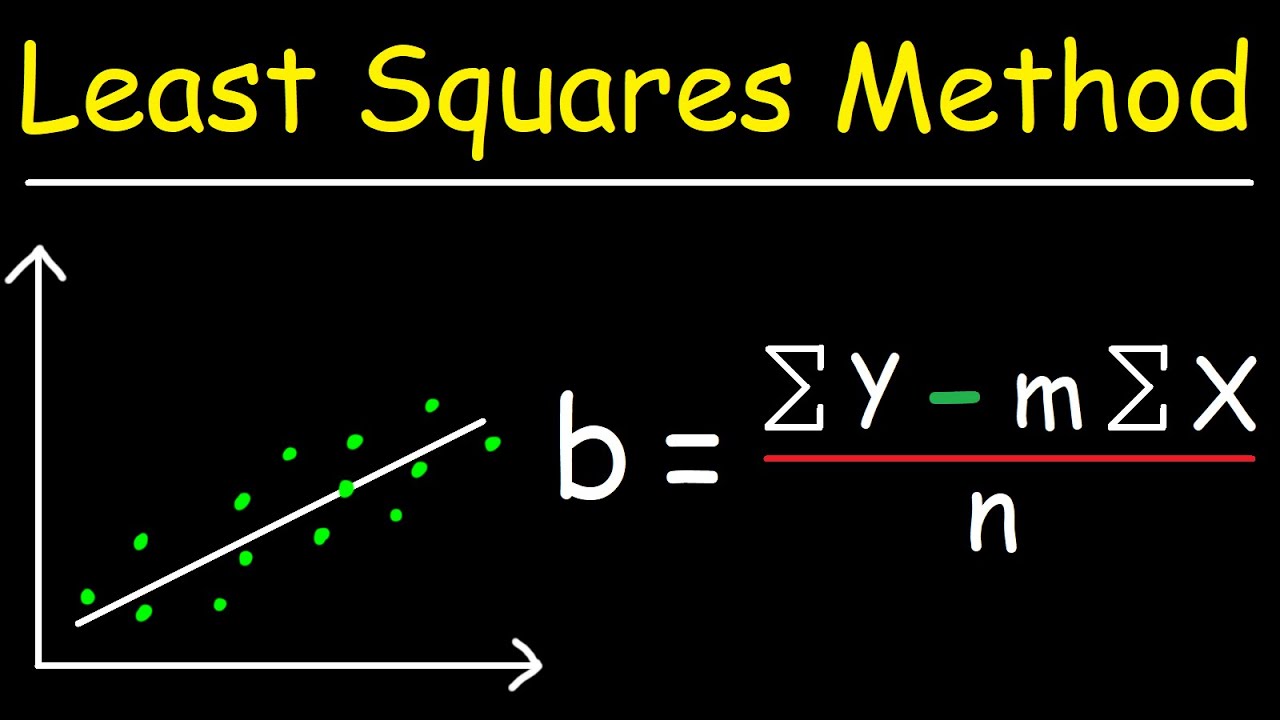
Understanding the Least Squares Method: A Simple Guide
The term “least squares method” sounds technical, but at its core it’s just a clever way to draw the best possible line through a cloud of data points. Whether you’re fitting a trend line to sales numbers or calibrating a sensor, the method helps you minimize the overall error between what you observe and what your model predicts.
What the Least Squares Method Actually Does
Imagine you have a scatter plot of measured values and you want a straight line that represents the underlying relationship. The least squares approach calculates the line whose squared vertical distances from every point are as small as they can be. By squaring the errors, larger deviations get penalized more heavily, which steers the fit toward the overall center of the cloud rather than being skewed by a single outlier.
Why It’s Popular in Data Analysis
Three reasons keep the least squares method at the forefront of statistics and machine learning.
- Simplicity. The math reduces to solving a set of linear equations, a task most software packages handle in a split second.
- Interpretability. The resulting coefficients have clear meanings – the slope tells you how much the response changes per unit of the predictor.
- Flexibility. Though often introduced with straight lines, the method extends to polynomials, multiple predictors, and even nonlinear transformations after a simple re‑coding step.
Step‑by‑Step: Applying Least Squares to a Linear Fit
Let’s walk through a tiny example with three observations: (1,2), (2,3), and (3,5). The goal is to find a line y = mx + b that best matches them.
- Write down the error for each point: e_i = y_i – (mx_i + b).
- Square each error and add them up: S(m,b) = Σ e_i².
- Take partial derivatives of S with respect to m and b, set them to zero, and solve the resulting equations. This yields the normal equations:
m·Σx_i² + b·Σx_i = Σx_i y_i
m·Σx_i + n·b = Σy_i
Plugging in the numbers (Σx_i = 6, Σy_i = 10, Σx_i² = 14, Σx_i y_i = 23, n = 3) gives a system that solves to m ≈ 1.5 and b ≈ 0.33. The line y = 1.5x + 0.33 is the least‑squares fit for this tiny data set.
Common Pitfalls and How to Avoid Them
Even a straightforward technique can trip you up if you ignore a few practical details.
- Assuming linearity. If the true relationship curves, a straight‑line fit will systematically misrepresent the data. Consider polynomial or spline extensions.
- Neglecting outliers. Because errors are squared, a single rogue point can dominate the solution. Robust alternatives like least absolute deviations can be safer in such cases.
- Ignoring heteroscedasticity. When the variance of errors changes with the predictor, the ordinary least squares (OLS) estimates remain unbiased but lose efficiency. Weighted least squares assigns lower weight to noisy observations.
When to Reach for a Different Technique
If you find yourself wrestling with any of the issues above, it might be time to explore alternatives. Logistic regression, for example, replaces the linear output with a probability when the response is categorical. Ridge or Lasso regression adds a penalty term to shrink coefficients, which helps when you have many predictors and risk overfitting. And for time‑dependent data, autoregressive models capture the inherent temporal structure better than a static fit.
FAQ
Q: Does the least squares method only work with two variables?
A: No. While the classic illustration uses a single predictor, the underlying mathematics generalizes to any number of independent variables, producing what’s called multiple linear regression.
Q: Is it necessary to standardize variables before applying least squares?
A: Standardization isn’t required for the algorithm to work, but it can improve numerical stability and make the coefficients easier to compare, especially when the predictors are on vastly different scales.
Q: How does the method handle missing data?
A: Ordinary least squares cannot directly incorporate missing entries; you’ll need to either omit incomplete rows or apply imputation techniques before fitting the model.
Q: Can I use least squares for non‑numeric data?
A: The method itself operates on numbers, so categorical variables must first be encoded—commonly via dummy variables—so that the regression treats them as binary predictors.